
Watch the video and support me on YouTube!
The Convolutional Neural Networks
Convolutional neural networks also referred to as CNNs are the most used type of neural network and the best for any computer vision applications. Once you understand these, you are ready to dive into this field and become an expert! The Convolutional Neural Networks are a family of deep neural networks that uses mainly convolutions to achieve the task expected.
A … convolution?

A convolution. Image via Irhum Shafkat
As the name says, convolution is the process where the original image, which is our input in a computer vision application, is convolved using filters that detects important small features of an image, such as edges. The network will autonomously learn filters value that detect important features to match the output we want to have, such as the name of the object in a specific image sent as input. These filters are basically squares of size 3-by-3 or 5-by-5 so they can detect the direction of the edge: left, right, up, or down. Just like you can see in this image, the process of convolution makes a dot product between the filter and the pixels it faces. Then, it goes to the right and does it again, convolving the whole image. Once it’s done, these give us the output of the first convolution layer, which is called a feature-map. Then, we do the same thing with another filter, giving us many filter maps at the end. Which are all sent into the next layer as input to produce again many other feature maps, until it reaches the end of the network with extremely detailed general information about what the image contains.
Training a CNN
Training process. Image via 3Brown1Blue
Typically, to learn the parameters of the filters we used during convolutions, called weights, we use a technique called back-propagation. This technique basically requires to first do a forward propagation into your network. Meaning that you feed it one or more example(s) and have a prediction from it. Where the prediction is what you want your model to achieve, like telling you if the image you sent contains a cat or a dog. Then, you use a learning technique, in this case, the backpropagation technique. Calculating the error between our guess and the real answer we were supposed to have. Propagating this error throughout the network changing the weights of the filters based on this error. Once the propagated error reaches the first layer, another example is fed to the network and the whole learning process is repeated. Thus iteratively improving our algorithm.
The activation function
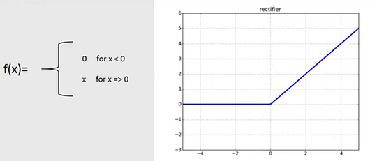
The ReLU activation function
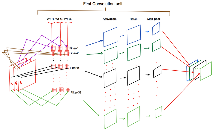
This activation function is responsible for determining the final output of each convolution computation and introduce non-linearities in our network, allowing it to model non-linear data. This way, it can stack convolutions and introduce the concept of “depth”, since stacking linear transformations is the same as having only one linear transformation. Thus, introducing this non-linearity is essential for our deep neural networks. The most popular activation function is called the ReLU function, which stands for Rectified Linear Unit. It is used right after a convolution inside what we call a “convolution unit”, or “conv”, as shown in the image below. It puts to zero any negative result making the convolution’s output more sparse, meaning that we have many zeros and a few important parameters. Thus “forcing” the network to focus on these parameters and be much more efficient to train in computation time, since a multiplication with zero, will always equal zero. It also helps to overcome the vanishing gradient problem, allowing models to learn faster and perform better, as we will discuss later.
The pooling layers
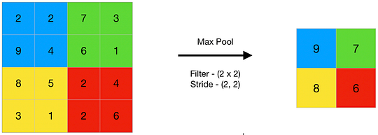
Max-Pooling. Image via GeeksForGeeks
Then, again to simplify our network and reduce the numbers of parameters, we have the pooling layers. Typically, we use a 2-by-2-pixels window and take the maximum value of this window to make the first pixel of our feature map. Then, we repeat this process for the whole feature-map, which will reduce the x-y dimensions of the feature-map, thus reducing the number of parameters in the network the deeper we get into it. This is all done while keeping the most important information.
These three layers, convolution, activation, and pooling layers can be repeated multiple times in a network, which we call our “conv” layers as shown in the image above, making the network deeper and deeper. Which is where the term “deep learning” comes from.

The final layers of a CNN architecture for computer vision
Finally, there are the fully-connected layers that learn a non-linear function from the last pooling layer’s outputs. Represented as the “FC” layers in the image below. It flattens the multi-dimensional volume that is resulted from the pooling layers into a 1-dimensional vector with the same amount of total parameters. Then, we use this vector in a small fully-connected neural network with one or more layers for image classification or other purposes resulting in one output per image, such as the class of the object. Of course, this is the most basic form of convolutional neural networks.
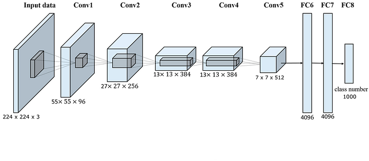
A basic CNN architecture for Imagenet object classification. Image via Andrew Gibiansky
The state-of-the-art CNNs
Quick history
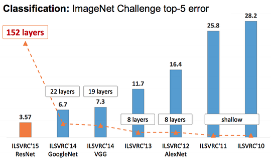
ILSVRC yearly results. Image via Prabhu
There have been many different convolutional architectures since LeNet-5 by Yann LeCun in 1998, and more recently with the first deep neural network applied in the most popular object recognition competition with the progress of our GPUs: the AlexNet network in 2012. This competition is the ImageNet Large Scale Visual Recognition Competition (ILSVRC), where the best object detection algorithms were competing every year on the biggest computer vision dataset ever created: Imagenet. It exploded right after this year. Where new architectures were beating the precedent one and always performing better, until today.
The most promising CNN architecture: DenseNet [1]
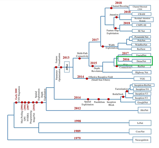
The history of CNNs. Image via A Survey of the Recent Architectures of Deep Convolutional Neural Networks
Nowadays, most state-of-the-art architectures perform similarly and have some specific use cases where they are better. You can see here a quick overview of the most powerful architectures. This is why I will only cover my favorite network in this article, which is the one that yields the best results in my researches, DenseNet. It is also the most interesting and promising CNN architecture in my opinion. Please, let me know in the comments if you would like me to cover any other type of network architecture!
The DenseNet family first appeared in 2016 in the paper called “Densely Connected Convolutional Networks” by Facebook AI Research. It is a family because it has many versions with different depths, ranging from 121 layers with 0.8 million parameters up to a version with 264 layers with 15.3 million parameters. Which is smaller than the 101 layers deep ResNet architecture!
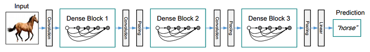
A deep DenseNet with three dense blocks. The layers between two adjacent blocks are referred to as transition layers and change feature-map sizes via convolution and pooling. Image via the DenseNet paper
As you can see here, the DenseNet architecture uses the same concepts of convolutions, pooling, and the ReLU activation function to work. The important detail and innovation in this network architecture are the dense blocks.
Here is an example of a five-layer dense block.
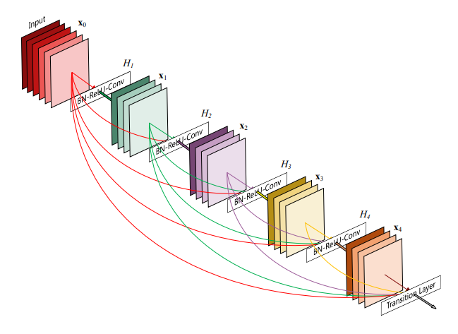
A 5-layer dense block. Each layer takes all preceding feature-maps as input. Image via the DenseNet paper
In these dense blocks, each layer takes all the preceding feature-maps as input, thus helping the training process by alleviating the vanishing-gradient problem. This vanishing-gradient problem appears in really deep networks where they are so deep that when we back-propagate the error into the network, this error is reduced at every step and eventually becomes 0. These connections basically allow the error to be propagated further without being reduced too much. These connections also encourage feature re-use and reduce the number of parameters, for the same reason, since it’s re-using previous feature-maps information instead of generating more parameters. And therefore accessing the network’s “collective knowledge” and reducing the chance of overfitting, due to this reduction in total parameters. And as I said, this works extremely well reducing the number of parameters by around 5 times compared to a state-of-the-art ResNet architecture with the same number of layers.
As you can see below, the original DenseNet family is composed of 4 dense blocks, with transition layers, which do convolution and pooling as well, and a final classification layer if we are working on an image classification task, such as the ILSVRC. The size of the dense blocks is the only thing changing for each version of the DenseNet family to make the network deeper.
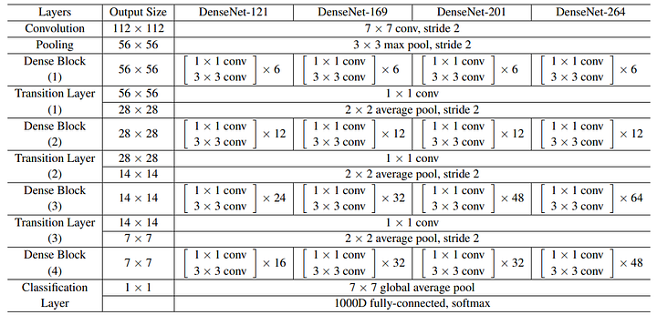
The DenseNet family. Image via the DenseNet paper
Conclusion
Of course, this was just an introduction to the convolutional neural networks and more precisely the DenseNet architecture. I strongly invite you to further read about these architectures if you want to make a well-thought choice with your application. The paper [1] and GitHub [2] links for DenseNet are below for more information. Please let me know if you would like me to cover any other architecture!
If you like my work and want to stay up-to-date with AI, you should definitely follow me on my other social media accounts (LinkedIn, Twitter) and subscribe to my weekly AI newsletter!
To support me:
- The best way to support me is by following me here on Medium or subscribe to my channel on YouTube if you like the video format.
- Support my work on Patreon
- Join our Discord community: Learn AI Together and share your projects, papers, best courses, find Kaggle teammates, and much more!
References
[1] G. Huang, Z.Liu, L. Maaten, k. Weinberger, Densely Connected Convolutional Networks (2016), https://arxiv.org/pdf/1608.06993.pdf
[2] G. Huang, Z.Liu, L. Maaten, k. Weinberger, Densely Connected Convolutional Networks — GitHub (2019), https://github.com/liuzhuang13/DenseNet